パトリック・シルベストル さん


バランスサンプリング(Cube法) [統計学]
効果的なサンプリング(標本抽出)について調べていたところ、バランスサンプリング(Cube法)という方法が良いらしいので早速試してみた。iAnalysisさんのブログ「調査のためのサンプリング」を参考にした。
■実験条件
1.データ
・MU284(アイスランドのデータ(税収、党の議席数など)-284件
2.R Package
sampling package
3.比較
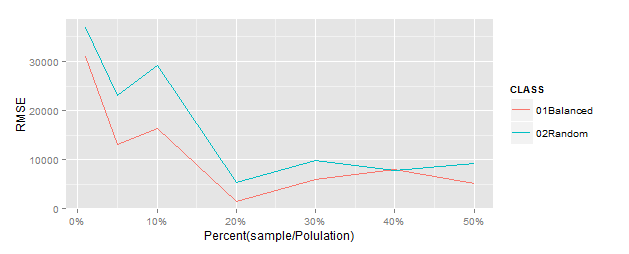
①Balanced SamplingとRandom Samplingについて変数:RMT85のHorvitz-Thompson推定量と全体合計との比較
②Balanced SamplingとRandom Samplingについてboxplotで比較
4.結果
①Horvitz-Thompson推定量と全体合計との比較
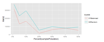
※Horvitz-Thompson推定量と全体合計のRMSEをプロット(この方法で検証あってるかちょっと不安)
②boxplotで比較
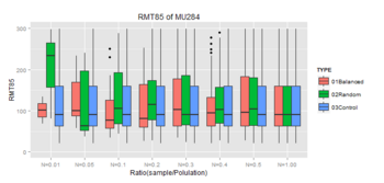
※Controlは母集団のBoxplot
★このデータの場合、バランスサンプリングは10%程度のサンプルで母集団との類似性が大きくなってきている。効果ありそう。もうちょっと調べてみようと思う。
6.コード
■参考文献
・概説 標本調査法 (統計ライブラリー)
")
cube法について書かれている和書はなさそうですが、標本調査の基礎にいてはこの本がわりと分かりやすいです。
・Sampling Algorithms (Springer Series in Statistics)
")
cube法について詳しく書いてあるのはこの本みたいです。本当にちゃんとやろうとすると洋書になっちゃうんですよね。やっぱり学者の層が薄いのでしょうか。いずれ読まなきゃなこの本。
■実験条件
1.データ
・MU284(アイスランドのデータ(税収、党の議席数など)-284件
2.R Package
sampling package
3.比較
①Balanced SamplingとRandom Samplingについて変数:RMT85のHorvitz-Thompson推定量と全体合計との比較
②Balanced SamplingとRandom Samplingについてboxplotで比較
4.結果
①Horvitz-Thompson推定量と全体合計との比較
※Horvitz-Thompson推定量と全体合計のRMSEをプロット(この方法で検証あってるかちょっと不安)
②boxplotで比較

※Controlは母集団のBoxplot
★このデータの場合、バランスサンプリングは10%程度のサンプルで母集団との類似性が大きくなってきている。効果ありそう。もうちょっと調べてみようと思う。
6.コード
####ライブラリ
library(sampling)
library(ggplot2)
library(scales)
data(MU284) #アイスランドのデータ(税収、党の議席数など)

#####サンプリング
###ランダムサンプリング関数
rsmpl <- function(DATA, i) {
  #i: 0 < i < 1
  nsample <- round(nrow(DATA)*i)
  p <<- rep(nsample/nrow(DATA), nrow(DATA))
  s <<- srswor(nsample, nrow(DATA))
  train <<- DATA[s==1, ]
  test <<- DATA[s==0, ]
}

####バランスサンプリング関数
csmpl <- function(X, DATA, i) {
  #i: 0 < i < 1
  nsample <- round(nrow(DATA)*i)
  p <<- rep(nsample/nrow(DATA), nrow(DATA))
  s <<- samplecube(X, p, 1, FALSE)
  train <<- DATA[s==1, ]
  test <<- DATA[s==0, ]
}
#csmpl(X, smpl, 0.01)

###サンプルと母集団の統計量比較
stat_comp <- function(sample, comp) {
  #出力したい変数に限定していると仮定
  rbind(summary(sample)[4, ], summary(comp)[4, ])
}
#stat_comp(train, smpl)

###Horvitz-Thompson 推定量
HT_comp <- function(sample, comp, pik, s) {
  HT <- HTestimator(sample, pik[s==1])
  CP <- sum(comp)
  RMSE <- sqrt((HT-CP)^2)
  R <<- data.frame(HT=HT, COMP=CP, RMSE=RMSE)
}
#HT_comp(train$age, smpl$age, p ,s)

####main()
###Test of Random Sampling
n <- c(0.01, 0.05, 0.1, 0.2, 0.3, 0.4, 0.5)
RSLT1 <- data.frame(HT=NULL, COMP=NULL, RMSE=NULL)
for(i in 1:length(n)) {
  rsmpl(MU284, n[i])
  HT_comp(train$RMT85, MU284$RMT85, p, s)
  RSLT1 <- rbind(RSLT1, R)
}
TMP <- data.frame(Smpl=rep(281,7)*n, Pop=rep(281,7), PCNT=n)
RSLT1 <- cbind(TMP, RSLT1)

###Test of Balanced Sampling
n <- c(0.01, 0.05, 0.1, 0.2, 0.3, 0.4, 0.5)
RSLT2 <- data.frame(HT=NULL, COMP=NULL, RMSE=NULL)
X <-cbind(MU284$P75,MU284$CS82,MU284$SS82,MU284$S82,MU284$ME84,MU284$REV84)

for(i in 1:length(n)) {
  csmpl(X, MU284, n[i])
  HT_comp(train$RMT85, MU284$RMT85, p, s)
  RSLT2 <- rbind(RSLT2, R)
}
TMP <- data.frame(Smpl=rep(281,7)*n, Pop=rep(281,7), PCNT=n)
RSLT2 <- cbind(TMP, RSLT2)

####可視化
RSLT1$CLASS <- "02Random"
RSLT2$CLASS <- "01Balanced"
RSLT <- rbind(RSLT1, RSLT2)
RSLT$CLASS <- as.factor(RSLT$CLASS)

gg <- ggplot(RSLT, aes(x=PCNT, y=RMSE, colour=CLASS)) + geom_line()
gg <- gg + xlab("Percent(sample/Polulation)") +
      scale_x_continuous(labels = percent)
gg

####Box-plotで分布を比較
###Test of Random Sampling
n <- c(0.01, 0.05, 0.1, 0.2, 0.3, 0.4, 0.5)
RAND <- NULL
for(i in 1:length(n)) {
  rsmpl(MU284, n[i])
  tmp <- data.frame(n=rep(n[i], nrow(train)),
                    RMT85=train$RMT85,
                    class=rep(paste0("N=",n[i]), nrow(train)))
  RAND <- rbind(RAND, tmp)
}
tmp <- data.frame(n=rep(1.00, nrow(MU284)),
                  RMT85=MU284$RMT85,
                  class=rep("N=1.00", nrow(MU284)))
RAND <- rbind(RAND, tmp)

###Test of Balanced Sampling
n <- c(0.01, 0.05, 0.1, 0.2, 0.3, 0.4, 0.5)
BLNC <- NULL
X <-cbind(MU284$P75,MU284$CS82,MU284$SS82,MU284$S82,MU284$ME84,MU284$REV84)

for(i in 1:length(n)) {
  csmpl(X, MU284, n[i])
  tmp <- data.frame(n=rep(n[i], nrow(train)),
                    RMT85=train$RMT85,
                    class=rep(paste0("N=",n[i]), nrow(train)))
  BLNC <- rbind(BLNC, tmp)
}
tmp <- data.frame(n=rep(1.00, nrow(MU284)),
                  RMT85=MU284$RMT85,
                  class=rep("N=1.00", nrow(MU284)))
BLNC <- rbind(BLNC, tmp)

###Control
n <- c(0.01, 0.05, 0.1, 0.2, 0.3, 0.4, 0.5)
CNTR <- NULL

for(i in 1:length(n)) {
  tmp <- data.frame(n=rep(n[i], nrow(MU284)),
                    RMT85=MU284$RMT85,
                    class=rep(paste0("N=",n[i]), nrow(MU284)))
  CNTR <- rbind(CNTR, tmp)
}
tmp <- data.frame(n=rep(1.00, nrow(MU284)),
                  RMT85=MU284$RMT85,
                  class=rep("N=1.00", nrow(MU284)))
CNTR <- rbind(CNTR, tmp)

####可視化
###データ加工
RAND$TYPE <- "02Random"
BLNC$TYPE <- "01Balanced"
CNTR$TYPE <- "03Control"
BOXP <- rbind(RAND, BLNC)
BOXP <- rbind(BOXP, CNTR)
BOXP$class <- as.factor(BOXP$class)
BOXP$TYPE <- as.factor(BOXP$TYPE)

gg <-  ggplot(BOXP, aes(class, RMT85)) +
       geom_boxplot(aes(fill = TYPE)) +
       ylim(0, 300) + ggtitle("RMT85 of MU284") +
       xlab("Ratio(sample/Polulation)")
gg
■参考文献
・概説 標本調査法 (統計ライブラリー)
- 作者: 土屋 隆裕
- 出版社/メーカー: 朝倉書店
- 発売日: 2009/08
- メディア: 単行本
cube法について書かれている和書はなさそうですが、標本調査の基礎にいてはこの本がわりと分かりやすいです。
・Sampling Algorithms (Springer Series in Statistics)
Sampling Algorithms (Springer Series in Statistics)
- 作者: Yves Tillé
- 出版社/メーカー: Springer
- 発売日: 2010/11/19
- メディア: ペーパーバック
cube法について詳しく書いてあるのはこの本みたいです。本当にちゃんとやろうとすると洋書になっちゃうんですよね。やっぱり学者の層が薄いのでしょうか。いずれ読まなきゃなこの本。
2013-02-24 15:18
nice!(0)
コメント(1)
トラックバック(0)
<a href="https://www.skorium.com" rel="noopener" title="카지노사이트">카지노사이트</a>
<a href="https://thedropshippingnomad.com/" rel="noopener" title="카지노사이트">카지노사이트</a>
<a href="https://www.legumassociates.com" rel="noopener" title="카지노사이트">카지노사이트</a>
by 카지노사이트 (2020-10-29 09:53)